Regularization and Optimization
Overfitting
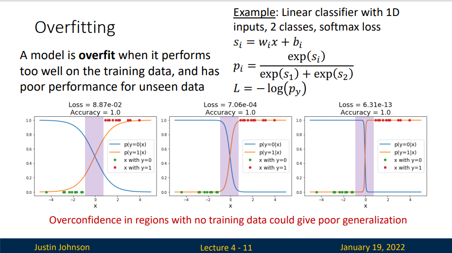
A model is overfit when it performs too well on the training data, and has poor performance for unseen data
Regularization
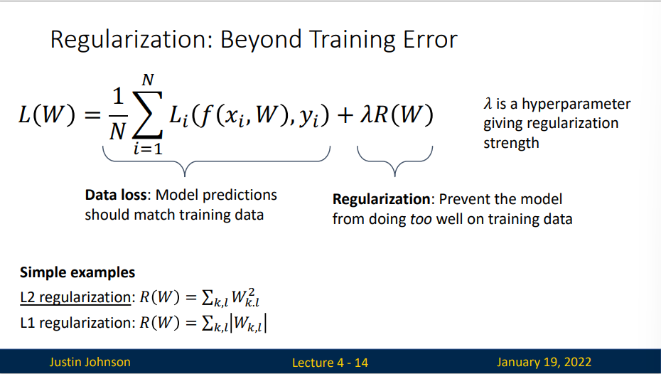
Loss function consists of data loss to fit the training data and regularization to prevent overfitting.
Optimization
最优化的目标就是找到能够最小化损失函数值的W。
Random Search
随机尝试很多不同的权重,看其中哪个最好
核心思路:迭代优化 :虽然找到最优化的权重W非常困难,但如果问题转化为:对一个权重矩阵集W取优,使其损失值稍微减少。那么问题的难度就大大降低了。换句话说,我们的方法从一个随机的W开始,然后对其迭代取优,每次都让它的损失值变得更小一点。
我们的策略是从随机权重开始,然后迭代取优,从而获得更低的损失值。
Follow the slope
In 1-dimennsion, the derivative of a function gives the slope:
In multiple dimensions, the gradient is the vector of (partial derivatives) along each dimension.
The slope in any direction is the dot product of the direction with the gradient. The direction of steepest descent is the negative gradient
Loss is a function of W: Analytic Gradient
- Numeric gradient: approximate, slow, easy to write
- Analytic gradient: exact, fast, error-prone
In pratice: Always use analytic gradient, but check implementation with numerical gradient. This is called a gradient check
Gradient Descent
Iteratively step in the direction of the negative gradient(direction of local steepest descent)
Hyperparameters - Weight initialization method - Number of steps - Learning rate \(\eta\)
学习率 \(\eta\) - 过小:下降速度缓慢,需要更多迭代次数,最终值与最优解存在偏差 - 过大:可能会发生overshoot
SGD
Batch Gradient Descent
Full sum expensive when N is large
如果使用梯度下降,每次自变量迭代的计算开销为 \(O(n)\),它随着\(n\)线性增长。因此,当训练数据样本(batch)数量很大时,梯度下降每次迭代的计算开销很高。 于是我们选取其中小批量\(N\)份数据样本(small batch)来计算梯度,实际中,\(N\)一般取32、64、128。显然他的计算开销为 \(O(N)\)。当批量较小时,每次迭代中使用的样本少,这会导致并行处理和内存使用效率变低。这使得在计算同样数目样本的情况下比使用更大批量时所花时间更多。当批量较大时,每个小批量梯度里可能含有更多的冗余信息。 当\(N=1\)时,该算法便是随机梯度算法
Hyperparameters: - Weight initialization - Number of steps - Learning rate - Batch size - Data sampling
Batch Size(一次训练所选取的样本数)的大小影响模型的优化程度和速度。同时其直接影响到GPU内存的使用情况,假如你GPU内存不大,该数值最好设置小一点。
- 设置合适时优点
- 通过并行化提高内存的利用率。就是尽量让你的GPU满载运行,提高训练速度。
- 单个epoch的迭代次数减少了,参数的调整也慢了,假如要达到相同的识别精度,需要更多的epoch。
-
适当Batch Size使得梯度下降方向更加准确。
-
从小到大的变化对网络影响
- 没有Batch Size,梯度准确,只适用于小样本数据库
- Batch Size=1,梯度变来变去,非常不准确,网络很难收敛。
- Batch Size增大,梯度变准确,
- Batch Size增大,梯度已经非常准确,再增加Batch Size也没有用 注意:Batch Size增大了,要到达相同的准确度,必须要增大epoch。
Stochastic Gradient Descent(SGD)
随机梯度下降减少了每次迭代的计算开销。在随机梯度下降的每次迭代中,我们随机均匀采样一个样本来计算梯度以迭代\(x\)。此时计算开销为\(O(1)\),同时我们也能可以看出随机梯度\(\nabla f_i(x)\)是对\(\nabla f(x)\)的无偏估计
Problems:
- What if loss changes quickly in one direction and slowly in another?
- Very slow progress along shallow dimension, jitter along steep direction
- What if the loss function has a local minimum or saddle point
- Zero gradient, gradient descent gets stuck.
- Our gradients come from minibatches, so the can be noisy
从迭代的次数上来看,SGD迭代的次数较多,在解空间的搜索过程看起来很盲目。
在以前,将梯度下降应用到非凸优化问题被认为很鲁莽或者没有原则。而现在,在深度学习中,使用梯度下降的训练效果很不错。虽然优化算法不一定能保证在合理的时间内达到一个局部最小值,但它通常能及时地找到代价函数一个很小的值,并且是有用的。
在深度学习之外,随机梯度下降有很多重要的应用。它是在大规模数据上训练大型线性模型的主要方法。对于固定大小的模型,每一步随机梯度下降更新的计算量不取决于训练集的大小m。在实践中,当训练集大小增长时,我们通常会使用一个更大的模型,但是这并非是必须的。达到收敛模型所需的更新次数通常会随着训练集规模增大而增加。然而,当m趋于无穷大时,该模型最终会随机梯度下降抽样完训练集上所有样本之前收敛到可能的最优测试误差。继续增加m不会延长达到模型可能的最优测试误差的时间。从这点来看,我们可以认为用SGD训练模型的渐进代价是关于m的函数的O(1)级别。
Momentum
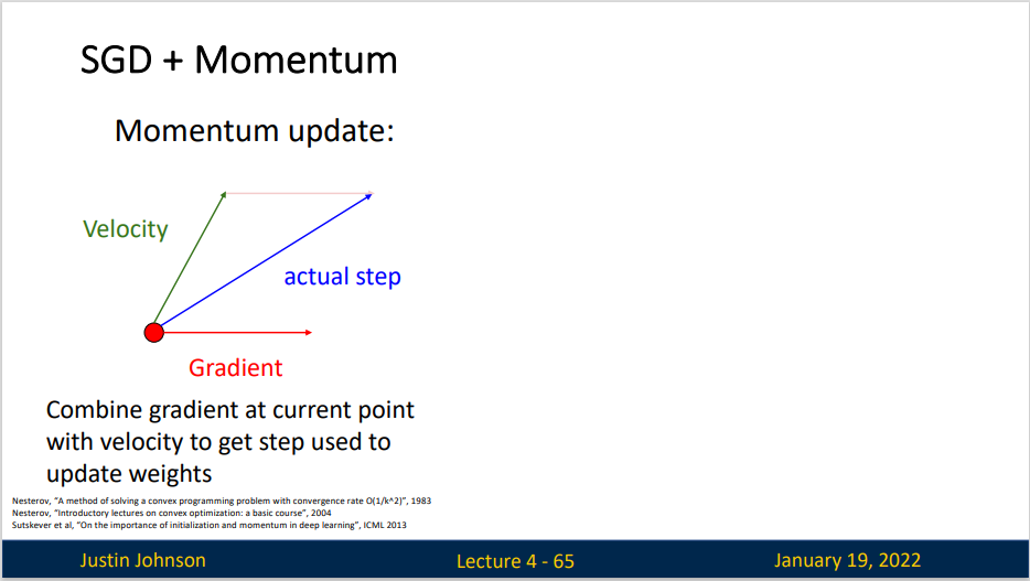
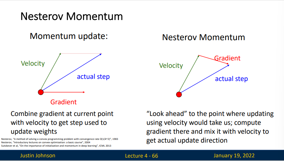
SGD+Momentum formulated different ways, but they are equivalent--give same sequence of x
| Python | |
|---|---|
| Python | |
|---|---|
动量积攒了历史的梯度,假定P点前一刻的梯度与当前的梯度方向几乎相反。因此原本在P点原本要大幅徘徊的梯度,主要受到前一时刻的影响,而导致在当前时刻的梯度幅度减小。
直观上讲就是,要是当前时刻的梯度与历史时刻梯度方向相似,这种趋势在当前时刻则会加强;要是不同,则当前时刻的梯度方向减弱。
或者说,要是当前时刻的梯度与历史时刻梯度方向相似,这种趋势在当前时刻则会加强;要是不同,则当前时刻的梯度方向减弱。
Nesterov Momentum
AdaGrad
为了获得良好的准确性,我们大多希望在训练过程中降低学习率,速度通常为 \(O(t^{-\frac{1}{2}})\)或更低。当某些不常见的特征(稀疏特征)出现时,与其相关的参数才会得到有意义的更新。鉴于学习率下降,我们可能最终会面这样情况:常见特征参数相当迅速地收敛到最佳值,而对于不常见地特征,我们仍缺乏足够地观测以确定其最佳值。换句话说,学习率要么对于常见特征而言降低太慢,要么对于不常见特征而言降低太快。
一个方法便是记录我们看到特定特征地次数,然后将其用作调整学习率
python
 grad_squared = 0
 for t in range (num_steps):
     dw = compute_gradient(w)
     grad_squared += dw*dw
     w -= learning_rate *dw / (grad_squared.sqrt()+1e-7)
这有两个好处:首先,我们不再需要决定梯度何时算足够大。 其次,它会随梯度的大小自动变化。通常对应于较大梯度的坐标会显著缩小,而其他梯度较小的坐标则会得到更平滑的处理。
缺点: 使得学习率过早,过量的减少
RMSProp
RMSProp算法是将速率调度与坐标自适应学习率分离的简单修复方法
python
 grad_squared = 0
 for t in range (num_steps):
     dw = compute_gradient(w)
     grad_squared = decay_rate*grad_squared + (1-decay_rate) *dw *dw
     w -= learning_rate *dw / (grad_squared.sqrt()+1e-7)
$$
r \leftarrow \rho r +(1-\rho )g \odot g
$$
由于神经网络都是非凸条件下的,RMSProp在非凸条件下结果更好,改变梯度累积为指数衰减的移动平均以丢弃遥远的过去历史。
- RMSProp算法与Adagrad算法非常相似,因为两者都使用梯度的平方来缩放系数。
- RMSProp算法与动量法都使用泄漏平均值。但是,RMSProp算法使用该技术来调整按系数顺序的预处理器。
- 在实验中,学习率需要由实验者调度。
- 系数\(\rho\)决定了在调整每坐标比例时历史记录的时长。
Adam RMSProp + Momentum
Adam算法的关键组成部分之一是:它使用指数加权移动平均值来估算梯度的动量和二次矩,即它使用状态变量
这里\(\beta_1\)和\(\beta_2\)是非负加权参数。 常将它们设置为\(\beta_1=0.9\)和\(\beta_2=0.999\)。 也就是说,方差估计的移动远远慢于动量估计的移动。
回顾Adam算法,它的设计灵感很清楚: 首先,动量和规模在状态变量中清晰可见, 它们相当独特的定义使我们移除偏项(这可以通过稍微不同的初始化和更新条件来修正)。 其次,RMSProp算法中两项的组合都非常简单。 最后,明确的学习率使我们能够控制步长来解决收敛问题。
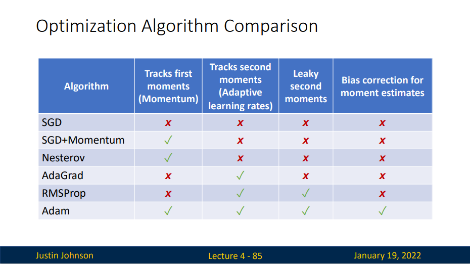
Comparison
First-Order and Second-Order
First-Order Optimization 1. Use gradient to make linear approximation 2. Step to minimize the approximation
Second-Order Optimization 1. Use gradient and Hessian to make quadratic approximation 2. Step to minimize the approximation
adaptively choose how big it should step
Seconde-Order Taylor Expansion:
Solving for the critical point we obtain the Newton parameter update:
- Quasi-Newton methods (BGFS most popular): instead of inverting the Hessian (\(O(n^3)\)), approximate inverse Hessian with rank 1 updates over time (\(O(n^2)\) each).
-
L-BFGS (Limited memory BFGS): Does not form/store the full inverse Hessian
-
Usually works very well in full batch, deterministic mode i.e. if you have a single, deterministic f(x) then L-BFGS will probably work very nicely
-
Does not transfer very well to mini-batch setting. Gives bad results. Adapting second-order methods to large-scale, stochastic setting is an active area of research
-
Adam is a good default choice in many cases SGD+Momentum can outperform Adam but may require more tuning
- If you can afford to do full batch updates then try out L-BFGS (and don’t forget to disable all sources of noise
Summary
- Use Linear Models for image classification problems
- Use Loss Functions to express preferences over different choices of weights
- Use Regularization to prevent overfitting to training data
- Use Stochastic Gradient Descent to minimize our loss functions and train the model